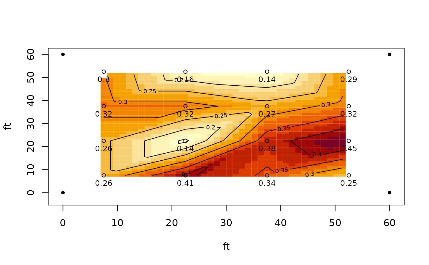
Plot a plan view of sprinklers and catch cans with collected depths.

plots a densigram with optional contour plot of catch can depths, with an option to label points. Both contour and point labeling are invoked by default (TRUE).

plotss(cdata,sploc,con=TRUE,xlab=NULL,ylab=NULL,xlim=NULL,
ylim=NULL,main=NULL,labelpoints=TRUE,pos=1,spklab=NULL,
pch=16,cex=0.8,edastat=FALSE,...)

Arguments

cdata

n x 3 matrix of catch can data; 1st column x, 2nd column y can locations, 3rd column catch depths

sploc

n x 2 matrix of sprinkler location data; 1st column xi, second column yi. i=4 for 4 sprinklers with cans in-between.

con

Logical; TRUE to overlay contour plot on densigram.

xlab

label for x axis of plot.

ylab

label for y axis of plot.

xlim

bounds of x-axis.

ylim

bounds of y-axis.

main

main title for plot.

labelpoints

logical; plot amounts at can locations? Default is TRUE.

pos

if labelpoints=TRUE, position of point labels, see text

spklab

character vector of labels for sprinklers. Defaults to bold italic to distinguish from can labels.

pch

symbol type. See par.

cex

scaling factor for plotting points and point labels.See par.

edastat

Logical; call eda.stat function for stats on catch depths?

...

further graphical parameters to pass to internal calls to plot.default

Value

densigram (from interp with optional contour plot overlay) and optional summary catch can statistics. Returned object is par(usr) to obtain x,y user coordinates for scaling subsequent plotting of low level plot functions on plotted densigram.

Author

Garry Grabow glgrabow@ncsu.edu

Note

requires interp package

See also

interp, contour

Examples

# set sprinkler locations (ft here)
sprinklerx<-c(0,0,60,60)
sprinklery<-c(60,0,60,0)
sploc<-cbind(sprinklerx,sprinklery)
#construct can data matrix
gage.space<-15
x<-c(rep(7.5,4),rep(22.5,4),rep(37.5,4),rep(52.5,4))
y<-rep(seq(52.5,7.5,-gage.space),4)
depth<-c(0.3,0.32,0.26,0.26,0.16,0.32,0.14,0.41,
0.14,0.27,0.38,0.34,0.29,0.32,0.45,0.25)
cdata<-cbind(x,y,depth)
plotss(cdata,sploc,xlab="ft",ylab="ft")

#> [1] -2.7 62.7 -5.4 62.7
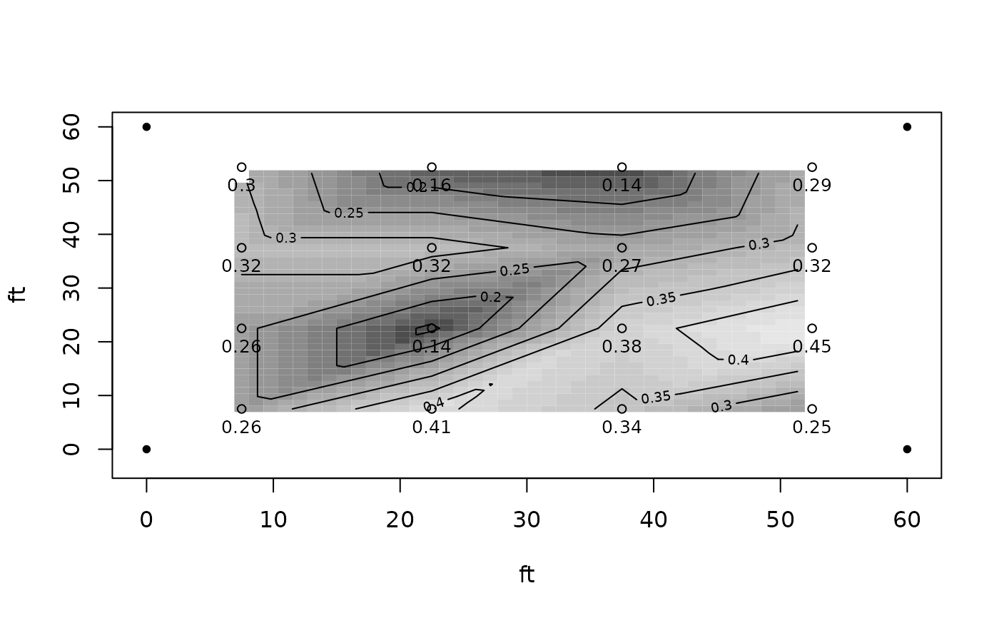
#now grey scale colors, pass "col"
plotss(cdata,sploc,xlab="ft",ylab="ft",col=grey.colors(16))

#> [1] -2.7 62.7 -5.4 62.7