Description
Lateral-move irrigation systems as defined here refer to sprinkler systems with laterals that are not “fixed” permanently in one position as with “solid set systems” but rather are “periodic-move” systems. In these systems one or more laterals is charged with flow to supply flow and pressure to sprinklers on the operating laterals. After an irrigation “set” is complete, the lateral is moved to another location for a subsequent irrigation. These systems reduce system capital costs (and pump costs) as compared to solid-set systems by limiting the number of laterals and sprinklers. An irrigation on a tract of land is accomplished by moving the laterals in irrigation “sets” across the field such that they are returned to their original positions by the time the next irrigation cycle is required. Example types of these systems are “hand-move” and “wheel-move” systems. Normally the laterals are moved in a direction perpendicular to a lateral, but some systems use hose-fed laterals with non-overlapping sprinklers, that are pulled in the lateral direction for achieving full coverage and overlap along the laterals in subsequent sets.
Because of their unique layout, lateral-move irrigation systems are evaluated for performance and uniformity in a slightly different manner than with a solid set, or hose-pull irrigation system.
Example
Data for this example are taken from the catchcan dataset. This data set contains catch can data for three types of sprinkler systems. The dataset for our lateral move example looks like this:
| l4 | l3 | l2 | l1 | r1 | r2 | r3 | |
|---|---|---|---|---|---|---|---|
| r1 | 0.10 | 0.21 | 0.24 | 0.28 | 0.23 | 0.21 | 0.03 |
| r2 | 0.11 | 0.21 | 0.26 | 0.31 | 0.31 | 0.16 | 0.01 |
| r3 | 0.10 | 0.16 | 0.22 | 0.32 | 0.31 | 0.15 | 0.04 |
| r4 | 0.10 | 0.23 | 0.27 | 0.32 | 0.27 | 0.17 | 0.03 |
| r5 | 0.08 | 0.20 | 0.25 | 0.30 | 0.35 | 0.19 | 0.03 |
| r6 | 0.06 | 0.16 | 0.19 | 0.33 | 0.27 | 0.11 | 0.04 |
where the columns labeled “l” show catch can collection rates (in/hr) to the left of the lateral (plan view) and those labeled with “r” are right of the lateral. A better view of the data from the single lateral trial can be performed using speval::plotss.
x<-seq(-35,25,10) # x=0 is lateral position. 10 x 10 catch can spacing
y<-seq(55,5,-10)
grd<-list(x,y) # prepare list for make.surface function [fields]
grid<-fields::make.surface.grid(grd)
rates<-matrix(t(cc.data),ncol=1)#transpose matrix and stack rows into 1 column
cdata<-cbind(grid[ ,1],grid[ ,2],rates) #construct required catch can data matrix
sp.x<-rep(0,3);sp.y<-seq(0,60,30)# sprinkler spacing (y) = 30 ft
sploc<-cbind(sp.x,sp.y) #construct required sprinkler location matrix
spr.lab<-c("s4","s5","s6")# labels for sprinklers
plotss(cdata,sploc,spklab=spr.lab)# call function
#> [1] -38  28  -6  63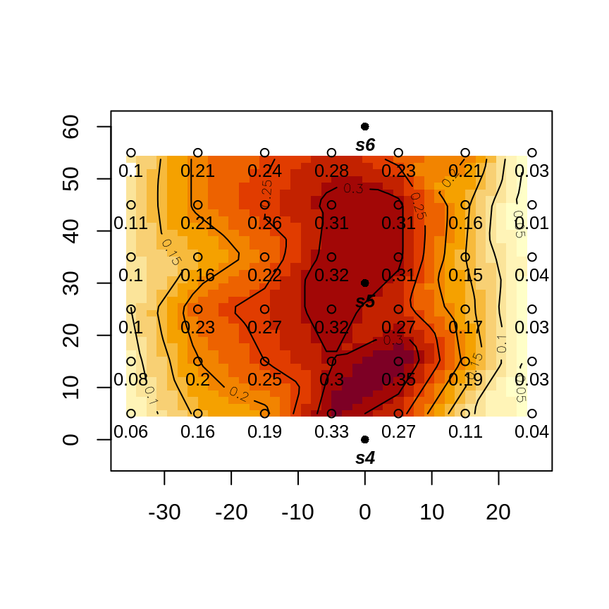
Raw catch can data, in./hr
In the figure above, the solid black dots at the upper, middle, and lower part of the plot at x=0 are the sprinkler locations along the single lateral, so in this test, data is from 3 sprinklers contributing to the catch cans indicated by open circle symbols. The 4 columns of catch cans to the left of the lateral, and only 3 to the right, are indicative of a prevailing wind from the upper right of the figure.
To evaluate sprinkler system uniformity, it is necessary to take account for operation of the lateral adjacent to the lateral operated for the test. This is done by overlapping, or superimposing the data from the one operating lateral as if an adjacent lateral was operating, or in the case of a periodic-move system, what would be expected from the next irrigation set with the lateral moved to a new position. The function speval::overlap is useful for superimposing the test data to simulate adjacent lateral operation for subsequent evaluation. speval::overlap operates using one “row” of can data from both left and right of the lateral; so overlap will need to be called for each row of catch can data. In this first case, a 50 ft lateral spacing will be used in the overlap process.
sl<-50 # 50 ft lateral spacing (pass to overlap)
sc<-10 # 10 ft catch can spacing perpindicular to lateral (pass to overlap)
#split data into left and right of lateral
left<-cc.data[ ,1:4];right<-cc.data[ ,5:7]#first 4 columns left of lateral
super.l=matrix(data=NA,nrow=nrow(left),ncol=sl/sc) # columns will be limited to between 2 adjacent laterals
super.r=matrix(data=NA,nrow=nrow(right),ncol=sl/sc)
for (i in 1:nrow(left)){
  lcdata<-rev(left[i,]);rcdata<-right[i, ]#overlap requires order from proximal lateral  to distal so rev (left)
  super<-overlap(sl,sc,lcdata,rcdata)
  super.l[i, ]<-super$sum.left;super.r[i, ]<-super$sum.right
}
knitr::kable(super.l,format="html")| 0.28 | 0.24 | 0.24 | 0.31 | 0.23 |
| 0.31 | 0.26 | 0.22 | 0.27 | 0.31 |
| 0.32 | 0.22 | 0.20 | 0.25 | 0.31 |
| 0.32 | 0.27 | 0.26 | 0.27 | 0.27 |
| 0.30 | 0.25 | 0.23 | 0.27 | 0.35 |
| 0.33 | 0.19 | 0.20 | 0.17 | 0.27 |
knitr::kable(super.r,format="html")| 0.23 | 0.31 | 0.24 | 0.24 | 0.28 |
| 0.31 | 0.27 | 0.22 | 0.26 | 0.31 |
| 0.31 | 0.25 | 0.20 | 0.22 | 0.32 |
| 0.27 | 0.27 | 0.26 | 0.27 | 0.32 |
| 0.35 | 0.27 | 0.23 | 0.25 | 0.30 |
| 0.27 | 0.17 | 0.20 | 0.19 | 0.33 |
Note that superimposing from right to left or left to right makes no difference other than being a mirror image. Either resultant matrix can be used to evaluate uniformity and other performance measures. This overlapped data can now be processed and plotted as with the original data using speval::plotss.
x<-seq(5,45,10) # x=0 is lateral position; look at right of test lateral
y<-seq(55,5,-10) # start at "top" y position, as a matrix
grd<-list(x,y) # prepare list for make.surface function [fields]
grid<-fields::make.surface.grid(grd)
o.rates<-matrix(t(super.r),ncol=1)#transpose matrix and stack rows into 1 column
o.cdata<-cbind(grid[ ,1],grid[ ,2],o.rates) #construct required catch can data matrix
sp.x.o<-c(sp.x,rep(50,3));sp.y.o<-c(sp.y,seq(0,60,30))#add second lateral location for overlap
sploc.o<-cbind(sp.x.o,sp.y.o) #sprinkler location matrix
spr.lab<-rep(c("s4","s5","s6"),2)# labels for sprinklers
plotss(o.cdata,sploc.o,spklab=spr.lab)# call function
#> [1] -3 53 -6 63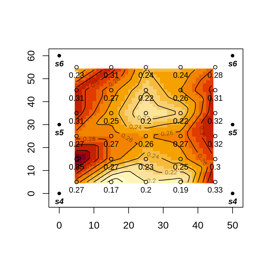
Overlapped catch can data rates (in./hr) at 50 ft lateral spacing
Note that the uniformity is improved by accounting for overlap of adjacent laterals.
Now we can use some measures of application uniformity and efficiency, specifically Christiansen’s coefficient of uniformity, distribution uniformity (of low quarter), distribution uniformity of the low half, and potential efficiency of the low quarter using the respective functions CU, DU, DU.lh and PELQ. We will divide the overlapped data set into 2 portions: the catch can data between sprinklers 4 and 5 (lower), and those between 5 and 6 (upper).
lower<-super.r[4:6,];upper<-super.r[1:3,]#use superimposed data
upper.uni<-c(CU(upper),DU(upper),DU.lh(upper),PELQ(upper,SI=FALSE,rate=4.6,ss=30,sl=50,dur=1))# use U.S. cust. units
lower.uni<-c(CU(lower),DU(lower),DU.lh(lower),PELQ(lower,SI=FALSE,rate=4.6,ss=30,sl=50,dur=1))
table<-round(rbind(upper.uni,lower.uni),0)
knitr::kable(table,row.names=TRUE,col.names=c("CU","DU","DU.lh","PELQ"))| CU | DU | DU.lh | PELQ | |
|---|---|---|---|---|
| upper.uni | 87 | 82 | 88 | 74 |
| lower.uni | 86 | 75 | 87 | 67 |
Note that the results for the upper and lower inter-sprinkler areas differ slightly. This could be due to a number of reasons: for example, slight variation in sprinkler rotation speed, slight difference in wind, or slight differences in sprinkler operating pressure that would be expected from relative sprinkler distance from the mainline (friction loss) or elevation difference.
Lastly, the application efficiency of the low quarter not only takes into account uniformity of application but the amount of applied water that is stored in the soil. Whenever the irrigation (average applied depth) exactly satisfies the soil moisture depletion (SMD) in the low-quarter watered areas, AELQ=PELQ. Irrigation depths greater than low-quarter SMD result in values of AELQ < PELQ. We can use the speval::ALEQ function, and in our example, for which the SMD= 4.4 in., and the sprinkler discharge rate is 4.6 gpm, ALEQ equals 63%
It may be of interest to evaluate the impact of different lateral spacing, especially during design of another similar system, or if the current system has laterals attached to hydrants using hoses that allows for operation at different lateral spacing. Using the same data, and overlapping at different lateral spacings (this time for 40- and 60-ft lateral spacings). The overlapped catch can data is shown below.
| 0.33 | 0.42 | 0.27 | 0.28 |
| 0.42 | 0.37 | 0.27 | 0.31 |
| 0.41 | 0.31 | 0.26 | 0.32 |
| 0.37 | 0.40 | 0.30 | 0.32 |
| 0.43 | 0.39 | 0.28 | 0.30 |
| 0.33 | 0.27 | 0.23 | 0.33 |
| 0.23 | 0.21 | 0.13 | 0.21 | 0.24 | 0.28 |
| 0.31 | 0.16 | 0.12 | 0.21 | 0.26 | 0.31 |
| 0.31 | 0.15 | 0.14 | 0.16 | 0.22 | 0.32 |
| 0.27 | 0.17 | 0.13 | 0.23 | 0.27 | 0.32 |
| 0.35 | 0.19 | 0.11 | 0.20 | 0.25 | 0.30 |
| 0.27 | 0.11 | 0.10 | 0.16 | 0.19 | 0.33 |
The measures of application uniformity and efficiency can now be computed for these alternate lateral spacings:
| CU | DU | DU.lh | PELQ | |
|---|---|---|---|---|
| upper.uni | 85 | 81 | 86 | 72 |
| lower.uni | 86 | 79 | 86 | 70 |
| CU | DU | DU.lh | PELQ | |
|---|---|---|---|---|
| upper.uni | 75 | 61 | 75 | 55 |
| lower.uni | 69 | 51 | 69 | 46 |
and the AELQ for the 40- and 60-ft lateral spacings are 51% and 55% respectively. Note that the AELQ, that measures efficiency, is lower for the lesser 40 ft lateral spacing, in contrast to the better application uniformity for the 40 ft spacing. This is because the application rate at the closer lateral spacing is higher, therefore applying a greater depth (catch can) that is in excess of the soil moisture deficit (SMD) and which leads to deep percolation losses. For the 60-ft lateral spacing AELQ=PELQ, meaning that the system application efficiency is limited solely by the irrigation system uniformity. If the irrigation duration is reduced to 11.5 hr from 23.5 hr, there will be no excess irrigation and hence no deep percolation losses and AELQ will change to 72% and 55% based on observations between the 5th and 6th sprinklers for the 40- and 60-ft lateral spacings respectively. With this irrigation duration, both spacings are limited only by the irrigation system application uniformity, however, in the case of the 60 ft lateral spacing, the reduced duration will result in under-irrigation as AELQ was equal to PELQ for both irrigation durations.
References
Mirriam and Keller, 1978. Farm System Irrigation Evaluation: A Guide for Management. PP 41-43. Utah State University, Logan, Utah. (https://pdf.usaid.gov/pdf_docs/PNAAG745.pdf).