Description
Solid-set Sprinkler systems include both buried and surface systems that are “permanent” in that sprinkler laterals are fixed. This is in contrast to lateral-move sprinkler systems in which one or more laterals are moved for a subsequent irrigation. In order to reduce pump and mainline cost, solid-set systems are normally divided into zones so that the pumping requirement based on the peak use rate of the crop for the whole field matches the system requirement (flow rate) of the zone. In this way all zones can be operated sequentially over an irrigation event before the initial zone requires a subsequent irrigation. These systems are generally more expensive than lateral move or hose-pull traveling gun systems due to the installed infrastructure, but do allow greater flexibility in operation. These systems are typically found in higher value agriculture (fruit or nut trees) or in wastewater irrigation. Residential and commercial turf irrigation systems are similar, and the functions in spreval can be used for either application.
Example
Data for this example are taken from the catchcan dataset. This data set contains catch can data for three types of sprinkler systems. The dataset for our lateral move example looks like this:
| c1 | c2 | c3 | c4 | |
|---|---|---|---|---|
| r1 | 0.57 | 0.69 | 0.83 | 0.65 |
| r2 | 0.61 | 0.38 | 0.27 | 0.64 |
| r3 | 0.51 | 0.26 | 0.36 | 0.52 |
| r4 | 0.79 | 0.65 | 0.61 | 0.86 |
This is a plan view of catch can data (in.) collected between 4 sprinklers spaced at a 80 ft x 80 ft (lateral x sprinkler) spacing. The catch cans are spaced at 20 ft x 20 ft.
These data may be plotted along with the sprinkler locations as a contour and image plot for a better representation of application uniformity using speval::plotss. Here, the upper left sprinkler is given an arbitrary location of (0,0).
#x,y matrix 20 ft x 20 ft catch can spacing
x<-seq(10,70,20) # catch can x coordinates.
y<-seq(-10,-70,-20) #catch can y coordinates.
grd<-list(x,y) # prepare list for make.surface function [fields]
grid<-fields::make.surface.grid(grd)
depths<-matrix(t(cc.data),ncol=1)#transpose matrix and stack rows into 1 column
cdata<-cbind(grid[ ,1],grid[ ,2],depths) #construct required catch can data matrix (x,y, depth)
sp.x<-c(0,0,80,80);sp.y<-c(0,-80,0,-80)# sprinkler spacing 80 x 80 ft
sploc<-cbind(sp.x,sp.y) #construct required sprinkler location matrix
spr.lab<-c("s12","s22","s13","s23")# label sprinklers as in reference
plotss(cdata,sploc,spklab=spr.lab)# call function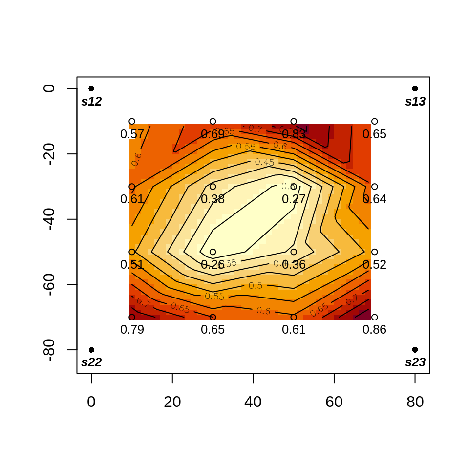
Raw catch can data, in.
In this example, there is no need to overlap test data, as with lateral-move and traveling gun system test data, to evaluate uniformity and efficiency.
Now we can use some measures of application uniformity and efficiency, specifically Christiansen’s coefficient of uniformity, distribution uniformity (of low quarter), distribution uniformity of the low half, and potential efficiency of the low quarter using the respective functions CU, DU, DU.lh and PELQ.
ss.uni<-c(CU(cc.data),DU(cc.data),DU.lh(cc.data),PELQ(cc.data,SI=FALSE,rate=16.98,ss=80,sl=80,dur=2.25))# use U.S. cust. units
table<-round(ss.uni,0)
knitr::kable(t(table),col.names=c("CU","DU","DU.lh","PELQ"))#transpose array (table) for display| CU | DU | DU.lh | PELQ |
|---|---|---|---|
| 75 | 55 | 76 | 55 |
Note that in the reference, the sprinkler discharge rate (which is a required parameter in PELQ)is not given. In this example, the sprinkler discharge rate (16.98 gpm) was simply calculated using the precipitation rate (in./hr) which is the average catch (in.) divided by the irrigation duration (2.25 hr), and the sprinkler and lateral spacing (80 ft x 80 ft). By using the average catch rate to obtain the precipitation rate, the PELQ exactly matches DU. The actual sprinkler discharge would be slightly greater, as drift and evaporation losses from the sprinklers to the catch cans would not be accounted for, and the PELQ would therefore be lower than in this example.
We can also look at the distribution of catch can depths using spreval::eda.shape
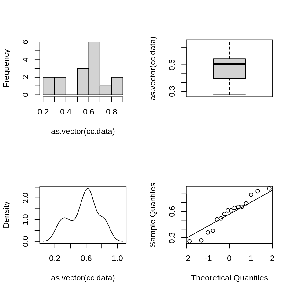
Distribution of catch can data in example
If a target depth is known, we can also compute percentile receiving depths lesser or greater than the target depth using speval::adper. This function uses both a density plot and empirical cumulative distribution function to determine the portion of catches above and below a given target depth.
results<-adper(cc.data,target=0.57)
headings<-c(results[[1]][1],results[[3]][1],results[[5]][1],results[[7]][1])#extract label elements
row.2<-c(results[[2]][1],results[[4]][1],results[[6]][1],results[[8]][1]) #extract value elements
adper.table<-rbind(headings,round(row.2,3))
knitr::kable(adper.table,row.names=FALSE,caption="adequacy and efficiency using density and cumulative distributions")| adequacy.density= | eff.density= | adequacy.ecdf= | eff.ecdf= |
| 0.557 | 0.443 | 0.562 | 0.438 |
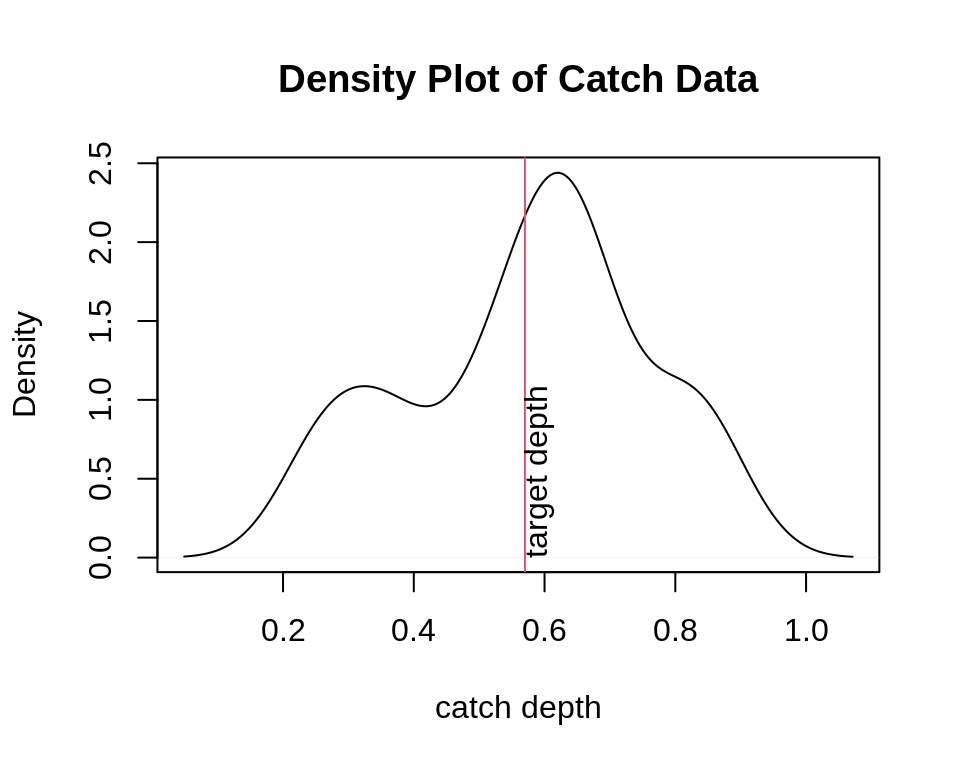
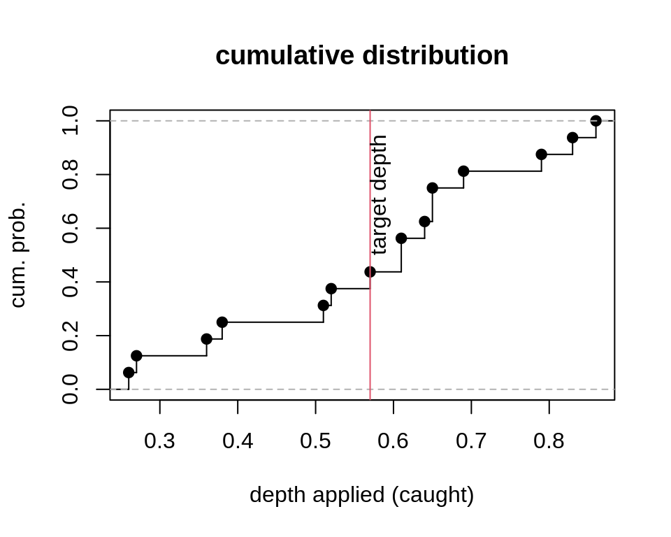
Percentile plot with target depth for example
Note that for either the “density” or “ecdf” plot approaches, the adequacy and efficiency values add to 1.0. With this function “adequacy” is simply the proportion of catches that receive depths equal to or greater than the target, while “efficiency” is defined at the proportion of catches that receive less than or equal to the target amount. Note also that this is not the standard definition of efficiency, in that it does not consider the difference in catch depths and the target depth, but only the proportion of depths less than or equal to the target depth. For a more traditional assessment of efficiency, we can use the function spreval::eff. This function uses a density plot to account for differences in catch depths from the target:
eff.table<-eff(cc.data,target=0.57)# call function
eff.table<-round(c(eff.table$appeff,eff.table$appadeq),3)
labels<-c("efficiency","adequacy")
eff.table<-cbind(labels,eff.table)
knitr::kable(eff.table)#| labels | eff.table |
|---|---|
| efficiency | 0.86 |
| adequacy | 0.868 |
A plot of an empirical cumulative distribution step function, rotated so that the soil surface is represented at the top of the plot, helps to visualize the above results. To do this, the function spreval::sfplot may be used.
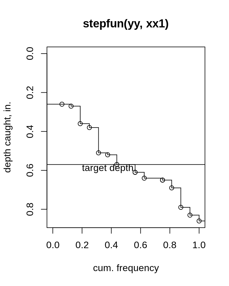
Rotated ECDF plot with target depth for example
The eff function integrates the area bounded by the catch depths and the target depth from a density plot and thus accounts for the deviation from the target depth and not just the relative number below and above the depth as with adper, and thus is a better measure of efficiency in the traditional sense. Using catch can data, however, does not account for losses between the sprinkler nozzle and the canopy or soil surface.
The target depth is usually the depth needed to refill the soil profile to field capacity, or in other words, the soil-moisture deficit (SMD) at the time of irrigation. As efficiency is traditionally defined as the amount of water applied that is stored in the root zone divided by the total amount of water applied, efficiency for a fixed applied irrigation depth can change depending on the initial SMD (target). To illustrate this we can run sfplot at different levels of SMD for the same fixed irrigation depth.
| targets | 0.40 | 0.50 | 0.60 | 0.70 |
| effic | 0.66 | 0.78 | 0.89 | 0.95 |
| adeq | 0.94 | 0.90 | 0.85 | 0.78 |
Notice how efficiency increases with increasing target depth (e.g., SMD) for this example irrigation that applied an average of 5.7 in (catch can average). Efficiency can approach 100% with deficit irrigation, but with greater efficiency comes reduced adequacy as can be seen in the table above.
References
Evans, R.O., Barker J.C., Smith J.T., Sheffield R.E. 1997a. Field calibration procedures for animal wastewater application equipment, stationary sprinkler irrigation system. NC Cooperative Extension Service publication AG 553-1. Raleigh, NC. (https://irrigation.wordpress.ncsu.edu/files/2017/01/ag-553-1-stationary-sprinkler.pdf).
Mirriam and Keller, 1978. Farm System Irrigation Evaluation: A Guide for Management. PP 41-43. Utah State University, Logan, Utah. (https://pdf.usaid.gov/pdf_docs/PNAAG745.pdf).